PPO보다 강력한 off policy 성격을 강화한 Policy Gradient!!!

ACER를 분석해 보자!!!

Policy Gradient는 기본적으로 on policy algorithm이다. TRPO, PPO는 on policy model이지만, off policy적인 요소를 반영했다. 여기서는 off policy 모델인 ACER의 구조와 구현에 대해서 살펴본다. 특히, 모델에 대한 설명을 구현을 고려한 관점에서 하고자 한다. 단순함을 위해, discrete action space만 고려한다.

개요

Sample Efficient Actor-Critic with Experience Replay. 2016년 11월, DeepMind.
simulation cost를 줄이기 위한 방안으로 sample efficiency를 높여야 한다. 그 방법 중에 하나가 replay memory(또는 replay buffer, experience replay)를 사용하는 것이다.
Actor Critic를 포함한 Policy Gradient(PG) 모델은 기본적으로 on policy 모델이다. PG가 replay memory를 사용할 수 있는 off policy가 될 수 없는 이유는 무엇일까?
replay memory에 쌓여 있는 action을 만들어낸 확률과 현재 train 대상이 되는 network이 만들어 내는 확률이 다르기 때문이다. train이 진행되면서 network이 update되기 때문이다. PG는 확률을 optimization해야 되는데, data의 reward를 얻게한 action의 확률은 현재의 network이 만들어내는 확률이 아니기 때문이다(gradient update를 통해 이미 변했기 때문).
이런 점 때문에, TRPO, PPO 모델에서는 data를 만들어낸 old policy와 train 대상이 되는 현재의 network의 new policy를 구분한다. (new policy는 network이 update되면서 계속 변한다). 그래서 new, old policy간 기대값 변환에 필요한 important sampling weight $\rho$가 필요하다. 또한 train이 되면서 계속 변하는 new policy가 data를 만들어낸 old policy로 부터 많이 벗어나지 못하게 제약을 주거나 trust region을 설정한다.
ACER에서는 PG모델에서 replay memory를 사용할 수 있는 방법을 제안하고 있다.
구현 코드는 OpenAI의 baselines을 참고하면 된다. 이 구현은 논문에 아주 충실하다.
Actor-Critic Model에서는 action 확률과 value를 예측하는 방식인데, ACER에서는 action 확률, action-value function $Q(x_t,a_t)$를 예측하고, 그 기대값인 $V(x_t)$도 사용한다.

\[\begin{eqnarray*} x_t &=& \text { state}, \ \ a_t = \text{ action} \\ \pi(a_t \vert x_t) &=& \text {모델이 추정한 action 확률}, \ \ \mu(a_{t}|x_{t}) = \text{ old policy 확률}\\ Q(x_t,a_t) &=& \text{모델이 추정한 action에 대한 $Q$ 값} \\ V(x_t) &=& \mathbb{E} [Q(x_t, a_t)] = \sum_{a_t} \pi(a_t|x_t) Q(x_t,a_t) \end{eqnarray*}\]

Replay Memory

replay memory를 사용하는 대표적인 모델이 DQN이다. DQN은 episode의 각 step이 하나의 data가 되고, 이것들이 모여서 replay momory를 이룬다.
ACER는 episode의 $k$-step개의 state, action, reward, done 등이 모여 하나의 data를 이룬다. $k$길이의 data들이 replay momory를 이룬다. mini-batch는 $k$길이의 data를 n개 선택하는 방식이다.

Retrace

on policy 모델인 PG에서는 (batch) data가 train 대상인 현재의 network으로부터 생성되었어야 하기 때문에, old policy로 생성된 data로 train을 할 수가 없다. 그래서 old policy로 생성된 $r_t$값을 train 대상이 되는 현재의 network이 예측한 $Q^\pi, V^\pi$로 보정해서 total gain $G_t$에 해당하는 $Q^{ret}$를 계산한다.
ACER 이전의 다른 Off Policy algorithm에서는 advantage 계산에 사용되는 $Q$값을 예측하기 위해서 lambda return 식을 제안하고 있다. (see T. Degris, M. White, and R. S. Sutton. Off-policy actor-critic. In ICML, pp. 457–464, 2012.)

\[R^{\lambda}_{t} = r_t + (1-\lambda)\gamma V(x_{t+1}) + \lambda \gamma \rho_{t+1} R^{\lambda}_{t+1}\]

This estimator requires that we know how to choose $\lambda$ ahead of time to trade off bias and variance. Moreover, when using small values of $\lambda$ to reduce variance, occasional large importance weights can still cause instability.
그래서 이 논문에서는 Retrace algorithm( see R. Munos, T. Stepleton, A. Harutyunyan, and M. G. Bellemare. Safe and efficient off-policy reinforcement learning. arXiv preprint arXiv:1606.02647, 2016.)을 사용하고자 한다.
Given a trajectory(episode path) generated under the behavior policy $\mu$(old policy), the Retrace estimator can be expressed recursively as follows($\lambda = 1$}:

\[Q^{ret}(x_t, a_t) = r_t + \gamma \bar{\rho}_{t+1} \Big[ Q^{ret}(x_{t+1}, a_{t+1}) - Q\pi(x_{t+1}, a_{t+1})\Big] + \gamma V(x_{t+1}),\]

where $\bar{\rho}_{t}$ is the truncated importance weight, $\bar{\rho}_{t} = \min \{c, \rho_t \}$ with $\rho_{t} = \frac{\pi(a_t\vert x_t) }{ \mu(a_t\vert x_t) }$.

Retrace is an off-policy, return-based algorithm which has low variance and is proven to converge (in the tabular case) to the value function of the target policy for any behavior policy.
좀 더 구체적으로, Retrace 계산과정을 살펴보자. trajectory $\{(x_t, a_t, r_t, d_t)\}_{t=1,\cdots,T}$와 $x_{T+1}$이 있어야 한다. 이로 부터

\[\big\{ ( r_t,d_t,\rho_t, V_t^{\pi}(x_t), Q_t^{\pi}(x_t,a_t) )\big\}_{t=1,\cdots,T}\]

와 $V_{T+1}^{\pi}(x_{T+1})$를 구한 후, $Q^{ret}$를 계산하게 된다. 각 계산은 batch 단위로 이루어질 수 있다.

다시 한번 정리해 보자.
1. $(r_t,d_t)$는 old policy에 의해 생성된 data.
2. $\rho_t$는 trajectory 사용된 old policy와 train대상이 되는 new policy의 action $a_t$에 대한 확률의 비율이다.
3. $\big(V_t^{\pi}(x_t), Q_t^{\pi}(x_t,a_t)\big)$는 new policy로 예측된 (traiable variable이 포함된) 값에서 trajectory data $(x_t,a_t)$에 해당하는 값이다.

참고로, OpenAI baselines 구현에서, $\bar{\rho}_{t} = \min \left\{c, \rho_t \right\}$에서 $c=1$이 사용되었다. 이제 $Q^{ret}$ 계산의 재귀적인 과정은 다음과 같다. $\begin{eqnarray*} z_{T+1} &=& V_{T+1}^{\pi} \\ Q^{ret}(x_T, a_T) &=& r_T + \gamma z_{T+1} (1-D_T) \ \ \ \leftarrow \text{$a_T$는 trajectory에 있는 action이다.} \\ z_{T} &=& \bar{\rho}_{T}\Big[ Q^{ret}(x_T, a_T) - Q^{\pi}(x_T, a_T) \Big] + V_T^{\pi} \\ &\vdots& \\ Q^{ret}(x_t, a_t) &=& r_t + \gamma z_{t+1} (1-D_t) \\ z_t &=& \bar{\rho}_{t} \Big[ Q^{ret}(x_t, a_t) - Q^{\pi}(x_t, a_t) \Big] + V_t^{\pi}\\ &\vdots& \end{eqnarray*}$

이렇게 계산된 $\{ Q^{ret}(x_t, a_t) \}$의 gradient는 backpropagation에 사용하지 않으며, Critic Network의 target 값이 된다.

Policy Gradient

이제 policy graident 식에 관해 살펴보자. $\pi$가 train 대상이 되는 new policy이고, $\mu$가 data를 생성한 old policy이다. 다음 2개의 식을 살펴보자. $\begin{eqnarray*} & & \mathbb{E}_{a_t \sim \mu} \Big[\rho_t \nabla_{\theta}\log \pi_\theta (a_t|x_t)Q^\pi(x_t, a_t)\Big] \\ &=& \mathbb{E}_{a_t \sim \mu} \Big[(\rho_t-c+c) \nabla_{\theta}\log \pi_\theta (a_t|x_t)Q^\pi(x_t, a_t)\Big] \nonumber\\ &=& \mathbb{E}_{a_t \sim \mu} \Big[c \nabla_{\theta}\log \pi_\theta (a_t|x_t)Q^\pi(x_t, a_t)\Big] + \mathbb{E}_{a_t \sim \mu} \Big[(\rho_t-c) \nabla_{\theta}\log \pi_\theta (a_t|x_t)Q^\pi(x_t, a_t)\Big] \nonumber\\ &=& \mathbb{E}_{a_t \sim \mu} \Big[c \nabla_{\theta}\log \pi_\theta (a_t|x_t)Q^\pi(x_t, a_t)\Big] + \mathbb{E}_{a_t \sim \pi} \Big[\frac{\rho_t-c}{\rho_t} \nabla_{\theta}\log \pi_\theta (a_t|x_t)Q^\pi(x_t, a_t)\Big] \end{eqnarray*}$

이 식과 다음 식은 같은 식이다.

\[\begin{eqnarray*} g_t^{marg} &=& \mathbb{E}_{a_t\sim\mu}\Big[ \bar{\rho}_{t} \nabla_{\theta} \log \pi_{\theta}(a_t \vert x_t) Q^\pi(x_t, a_t) \Big] + \underset{a \sim \pi}{\mathbb{E}} \Bigg( \Big[\frac{\rho_{t}(a) - c}{\rho_{t}(a)} \Big]_+ \hspace{-3mm} \nabla_{\theta} \log \pi_{\theta}(a\vert x_t) Q^\pi(x_t, a) \Bigg). \end{eqnarray*}\]

위의 2개 식이 같은 이유를 $\rho < c$인 경우와 $\rho \geq c$인 경우로 나누어 생각해 보면 알 수 있다.
1. $\rho_t < c$인 경우: 뒷부분이 없어진다. $\rho = \bar{\rho}_{t}$. 이렇게 되면, 두 식은 일치한다.
2. $\rho_t \geq c$인 경우: $\rho_{t} = c + \rho_t - c = \bar{\rho}_{t} + \big( \rho_{t} - c \big)$. 여기서 $\big( \rho_{t} - c \big)$를 $\rho_{t}$로 나누어 주고, old policy에서 new policy에 대한 기대값으로 전환하면 앞 식의 뒷부분이 된다. 따라서, 이 경우에도 두 식은 일치한다.
old policy에 대한 기대값이므로, off policy 환경에서 계산을 위하여 $Q^\pi$를 $Q^{ret}$로 대체하여 $\widehat{g}_t^{marg}$을 다음과 같이 정의한다.

\[\begin{eqnarray*} \widehat{g}_t^{marg} &=& \bar{\rho}_{t} \nabla_{\theta} \log \pi_{\theta}(a_t\vert x_t) Q^{ret}(x_t, a_t) + \underset{a \sim \pi}{\mathbb{E}} \Bigg( \Big[\frac{\rho_{t}(a) - c}{\rho_{t}(a)} \Big]_+ \hspace{-3mm} \nabla_{\theta} \log \pi_{\theta}(a \vert x_t) Q^\pi(x_t, a) \Bigg). \end{eqnarray*}\]

다시 Gain에 해당하는 부분을 Advantage로 변환하여 $\widehat{g}_t^{acer}$를 정의한다.

\[\begin{eqnarray*} \widehat{g}_t^{acer} &=& \bar{\rho}_{t} \nabla_{\theta} \log \pi_{\theta}(a_t \vert x_t) \overbrace{\big[Q^{ret}(x_t, a_t) - V^\pi(x_t)\big]}^{\text{stop gradient}} \\ && + \underset{a \sim \pi}{\mathbb{E}} \Bigg( \Big[\frac{\rho_{t}(a) - c}{\rho_{t}(a)} \Big]_+ \hspace{-3mm} \nabla_{\theta} \log \pi_{\theta}(a\vert x_t) \overbrace{\big[Q^\pi(x_t, a)- V^\pi(x_t)\big]}^{\text{stop gradient}} \Bigg). \end{eqnarray*}\]

이 $\widehat{g}_t^{acer}$가 ACER의 Trust Region을 적용하기 전의 gradient 식이 된다.

Loss 계산

Entropy Gain: $\pi(a_t|x_t)$는 모델이 추정한 action 별 확률 $\pi(\cdot|x_t) = (p_{t1}, p_{t2}, \cdots, p_{tn})$ 중에서 trajectory action $a_t$에 해당하는 값이다. Entropy Gain는 모든 확률 $(p_{t1}, p_{t2}, \cdots, p_{tn})$로부터 계산할 수 있다.

\[L_1 : = -\sum_i p_{ti} \log p_{ti}\]

Policy Loss: $\widehat{g}_t^{acer}$의 앞부분: $V^\pi(x_t) = \sum_{a} \pi(a|x_t) Q^\pi(x_t,a)$와 $\overbrace{Q^{ret}(x_t, a_t)}^{a_t\text{는 trajectory action}}$로 부터 advantage $A_t: =\underbrace{Q^{ret}(x_t, a_t)}_{\text{batch-size}} - \underbrace{V^\pi(x_t)}_{\text{batch-size}}$를 계산할 수 있고, 이로 부터 Policy Loss를 다음과 같이 구할 수 있다.

\[L_2 := \log \Big(\pi(a_t|x_t) \Big) \times \overbrace{A_t \times \min \big[ c, \rho_t(a_t) \big]}^{\text{stop gradient}} \ \ \ \leftarrow \text{ 각각이 batch-size}\]

여기서도 $A_t,\rho_t(a_t)$의 gradient는 계산하지 않는다. 또한 이 loss는 trajectory action을 기반으로 계산되었다. 다음에 나오는 Bias Correction은 모든 action 확률에 대한 기대값을 계산한다.

Bias Correction: $\widehat{g}_t^{acer}$의 뒷부분: 이 계산에 사용되는 advantage

\[A_t^{\text{bc}} = \underbrace{Q^\pi(x_t,\cdot)}_{\text{batch-size, action-size}} - \underbrace{V^\pi(x_t)}_{\text{batch-size}}\]

는 broadcasting을 적용하기 위해 $V^\pi(x_t)$를 reshape해야 한다.

\[L_3 :=\sum_{\text{성분}} \Bigg[(p_{t1}, p_{t2}, \cdots, p_{tn}) \circ \big[1-\frac{c}{\rho_{t}} \big]_+ \circ A_t^{\text{bc}} \circ (\log p_{t1}, \log p_{t2}, \cdots, \log p_{tn})\Bigg]\]

이 식은 확률이 곱해져 있으므로, 모든 성분을 합치면 기대값이 된다. 참고로, OpenAI baselines 구현에는 $L_2, L_3$에서 $c=10$이 사용되었다.

Value(Critic) Loss:

\[L_4 := \frac{1}{2}\Big\Vert Q^{ret}(x_t, a_t) - Q^\pi(x_t,a_t) \Big\Vert^2\]

여기서도 $Q^{ret}(x_t, a_t)$의 gradient는 계산하지 않는다.

total loss: loss weight $\lambda_1$(e.g. 0.01), $\lambda_4$(e.g. 0.5)에 대하여

\[\textbf{L} := -\lambda_1 L_1 + L_2 + L_3 + \lambda_4 L_4\]

Trust Region

Trust Region을 적용하지 않는다면, $\textbf{L}$을 최소화하기 위해, $\frac{\partial \textbf{L}}{\partial f}$를 계산하여 Gradient Descent를 적용하면 된다. 그런데, Trust Region을 적용한다면, $\frac{\partial \textbf{L}}{\partial f}$와 가깝지만, 어느 정도 조건을 만족하는 vector를 구해 대신하는 방식을 사용한다.
old policy 대신 moving average policy를 사용한다. $\Rightarrow$ `polyak(러시아 수학자) averaging라고 부르기도 한다. moving average policy로 부터의 action별 확률을 $f_{\text{pol}}$이라 하자.
일반적(TRPO)으로 모든 weight에 대한 $\textbf{L}$의 gradient에 제약을 하는데, ACER에서는 action 확률 $f:= \pi(\cdot|x_t)$에 대한 gradient에 제약을 주어 trust region을 적용한다. Loss $\textbf{L}$에서 $f$성분이 없는 $L_4$를 제외하고 gradient를 $\hat{g}^{acer}_t$를 다음과 같이 정의한다.

\[\hat{g}^{acer}_t: = \nabla_{f}\big(-\lambda_1 L_1 + L_2 + L_3\big) \ \ \ \ \Big(= \frac{\partial \textbf{L}}{\partial f} \leftarrow \text{(batch-size,action-size)}\Big)\]

$\hat{g}^{acer}_t$가 Loss minimization을 수행할 gradient인데, 이 $\hat{g}^{acer}_t$에 가까우면서 제약식을 만족하는 새로운 gradient $z$을 찾는 것이 우리가 하고자 하는 바이다.

$f$에 대한 KL divergence $D_{KL}(f_{\text{pol}} \Vert f)$의 gradient를 $k$로 정의하자.

\[k := \nabla_f D_{KL}(f_{\text{pol}} \Vert f) \ \ \ \leftarrow \text{(batch-size,action-size)}\]

이제 다음과 같은 optimization 식을 살펴보자.

\[\begin{aligned} & \underset{z}{\text{minimize}} & & \frac{1}{2}\| \hat{g}^{acer}_t - z\|^2_2 \\ & \text{subject to} & & k^T z \leq \delta \end{aligned}\]

제약식에서 $k$와 $z$의 내적이 $\delta$(e.g. 1)보다 작다는 의미를 생각해 보자. $k$는 KL Divergence의 $f$에 대한 gradient이다. 내적 값 $k^T z$가 일정한 값 $\delta$보다 작다는 것은 KL Divergence를 커지지 않게 하라는 의미이다. 이런 조건을 만족하는 $z$중에서 $\hat{g}^{acer}_t$에 가까운 $z$를 찾아 $\hat{g}^{acer}_t$를 대체하는 gradient로 $z$를 사용하려 한다. 이 optimization 문제는 KKT condition을 이용하면, 다음과 같은 closed form solution $z^*$를 가진다.

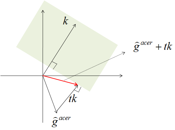
\[z^* = \hat{g}^{acer}_t - \max \Bigg\{ 0, \frac{k^T \hat{g}^{acer}_t - \delta}{\Vert k \Vert_2^2} \Bigg\}k \ \ \ \leftarrow\text{max값은 scalar값이므로, batch-size 크기.}\]

KL Divergence Optimization

*Fig. 1. 영역에 포함되면서 $\hat{g}^{acer}_t$에 가장 가까운 벡터를 찾는 문제이다. $k^T\big(\hat{g}^{acer}_t + tk\big)=\delta$인 $t$를 찾으면 된다. *

이런 접근이 장점만 있는 것은 아니다. 모든 weight의 gradient에 대한 제약식이 아닌, 중간 변수 $f$에 대한 제약식이므로, 계산량과 stability의 trade off가 생긴다.

\[\begin{eqnarray*} \frac{\partial \textbf{L}}{\partial \theta} &=& \frac{\partial \textbf{L}}{\partial f} \frac{\partial f}{\partial \theta} + \lambda_4\frac{\partial L_4}{\partial \theta} \\ &\approx& z^* \frac{\partial f}{\partial \theta} + \lambda_4\frac{\partial L_4}{\partial \theta} \end{eqnarray*}\]

참고로 $k = \nabla_f D_{KL}(f_{\text{pol}} \Vert f)$를 계산해 보자. KL Divergence는 $(\log f_{\text{pol}} - \log f)$를 확률 $f_{\text{pol}}$로 기대값을 계산하면 된다. 따라서 $(\log f_{\text{pol}} - \log f)$과 $f_{\text{pol}}$의 내적(scalar)을 $f$로 (정확히는, $f$의 각 성분 으로) 미분하면,

\[k = - \frac{ f_{\text{pol}}}{ f}\]

======================

구현 코드 분석

OpenAI의 baselines의 ACER 코드(Tensorflow)를 분석해 보자.
acer.py에 핵심적인 부분이 다 구현되어 있다.
OpenAI의 ACER 구현은 discrete action space만 구현되어 있다. continuous action 인 “Pendulum-V0” 같은 env는 작동하지 않는다.
OpenAI baselines는 MPI를 사용한다. Windows환경에서는 단순 pip만으로 mpi4py가 설치되지 않는다.

Policy Network

with tf.variable_scope('acer_model', reuse=tf.AUTO_REUSE):
	# policy = common/policies.py PolicyWithValue
	step_model = policy(nbatch=nenvs, nsteps=1, observ_placeholder=step_ob_placeholder, sess=sess)
	train_model = policy(nbatch=nbatch, nsteps=nsteps, observ_placeholder=train_ob_placeholder, sess=sess)

with tf.variable_scope("acer_model", custom_getter=custom_getter, reuse=True):
	polyak_model = policy(nbatch=nbatch, nsteps=nsteps, observ_placeholder=train_ob_placeholder, sess=sess)  # exponential weighted model

3개의 policy를 생성한다(episode 생성, train, exponential average). reuse=True 설정되어있고, polyak_model은 tf.train.ExponentialMovingAverage로 만들어진다.

Polyak Average

ema = tf.train.ExponentialMovingAverage(alpha)  # alpha=0.99
ema_apply_op = ema.apply(params)

def custom_getter(getter, *args, **kwargs):
	v = ema.average(getter(*args, **kwargs))
	print(v.name)
	return v

with tf.variable_scope("acer_model", custom_getter=custom_getter, reuse=True):
	# polyak averaging
	polyak_model = policy(nbatch=nbatch, nsteps=nsteps, observ_placeholder=train_ob_placeholder, sess=sess)  # exponential weighted model

이렇게 구현된 ema_apply_op는 optimization을 수행하는 train_op와 tf.control_dependencies로 묶으면 된다.

with tf.control_dependencies([train_op]):
	_train = tf.group(ema_apply_op)

train_op가 실행된 후, ema_apply_op가 실행되면서 polyak_model이 update된다.

On/Off Policy Train

for acer.steps in range(0, total_timesteps, nbatch): #nbatch samples, 1 on_policy call and multiple off-policy calls
	acer.call(on_policy=True)
	if replay_ratio > 0 and buffer.has_atleast(replay_start):
		n = np.random.poisson(replay_ratio)
		for _ in range(n):
			acer.call(on_policy=False)  # no simulation steps in this

train은 on-policy train 1번 후, off policy를 random하게 몇번 하는 방식으로 이루어진다.

on-policy train: data 생성한 후, replay buffer에 쌓고, 그 data로 train한다.

off-policy train: replay buffer에서 random하게 data를 뽑아서 train한다.

CartPole-v1 구현

Code
OpenAI baselines 코드는 여러 환경에서 작동하도록 설계되어, 알고리즘을 분석하기에는 좀 복잡하다.
baselines에서 ACER부분만 추출. MPI로 구현된 부분을 multiprocessing로 대체.

BreakoutDeterministic-v4 구현

Code
OpenAI baselines 코드를 simplel하게 수정
MPI 대신 multiprocessing으로 구현
Optimizer를 RMSProp 대신, Adam 사용
process 8개 사용.
learning_rate = 0.00025에서 출발하여 점차적으로 감소
2시40분 정도 train하면 적절. 좀 더 train하면 4시간 정도까지.

Reference

딥러닝 정리 자료
PPO, TRPO는 on policy인가, off policy인가? https://github.com/openai/baselines/issues/316